← All Work

Telecom · RAN Engineering 2024

RANSyncX

Building a Direction-Aware Neighbor Database for FWA Cell Locking

Role: Lead Developer / Data Scientist
Status: Ongoing

Pythonscikit-learnGeospatial AnalyticsRAN EngineeringNetwork Automation

Outcome

KNN (BallTree / NearestNeighbors) Candidate generation

Antenna-azimuth alignment Elimination logic

Four explainable tiers Priority output

~99% Database accuracy

The Original Requirement

FWA routers work off a locked list of cells — the base stations they're allowed to attach to. The existing logic for building that list started from the original CDR cells for a site, and an earlier stage had already extended it with collocated cells sitting on the same physical site.

The next requirement was to go further and add neighboring cells too — cells nearby but not on the same site — so the locked list could grow toward a pre-agreed cap of roughly 50 cells per site. That's where this project started: out of everything nearby, which cells actually belong on that list?

Starting With Proximity

The obvious first move was geographic nearest-neighbor search. I used sklearn.neighbors for this — BallTree and NearestNeighbors — to pull in the geographically closest cells around each target as candidates.

That part worked well and was fast enough to run across the network. But I want to be clear about what it actually gave me: a list of geographically close cells, nothing more. Nearest-neighbor search was candidate generation, not the final decision logic. Whether a candidate actually belonged in the neighbor set was a separate question I hadn't answered yet.

Why Distance Alone Wasn't Enough

The first version gave me geographically close cells, which was useful for narrowing the search space. But once I started checking the results against real sector layouts, the weakness became obvious: some of the closest cells were pointing away from the target entirely.

A cell can sit fifty meters from a site and still be useless as a neighbor, if its antenna sector faces the opposite direction. Distance alone can't tell you that. Adding every nearby candidate without checking direction would have polluted the neighbor database with cells that have no real radio relationship to the target — close on a map, irrelevant on the air interface.

That's the point where the question changed. It stopped being 'which cells are closest?' and became 'which nearby cells are also geometrically meaningful from a radio and antenna-direction perspective?'

Adding Antenna-Direction Reasoning

I kept KNN as the candidate-generation stage, but I stopped treating distance as the final decision. Each candidate cell has an antenna azimuth — the direction its sector actually points. I compared that against the bearing from the candidate cell toward the target, which is the direction you'd have to look to find the target from the candidate's position.

To compare the two, I converted both the azimuth and the bearing into unit direction vectors and used a dot-product comparison to measure how well they line up. The result is an angular difference in degrees: the smaller the difference, the more the candidate's antenna is actually pointed toward the target rather than just sitting nearby.

A candidate only survives if that angular difference falls under a configurable angular-alignment threshold. I kept the threshold as a parameter rather than a hardcoded constant, because what counts as 'close enough' can reasonably shift depending on the deployment and the antenna patterns involved.

Small angular difference Approved

Large angular difference Rejected

Illustrative angles, not measured data — the smaller the angle between the two vectors, the more the candidate's antenna is actually pointed at the target rather than just sitting nearby.

The Math Behind It

None of the above is qualitative — every step reduces to plain vector geometry, and every formula below sits right next to the real code that implements it, a few paragraphs down: distance and bearing first, then the direction vectors and the dot-product comparison they feed into.

How the Logic Works

def _run_pipeline(self, df: pd.DataFrame) -> pd.DataFrame:
    _df = self.compute_direction_vectors(df)
    _df = self.calculate_vector_and_angle_vectorized(_df)
    _df = self.evaluate_coverage_direction(_df)
    _df = self.assign_status(_df)
    return _df

I kept the elimination logic as a sequence of explicit geometric steps instead of one dense function — each step is independently testable and easy to reason about on its own.

Geodesic distance

d = geodesic( (lat₁, lon₁), (lat₂, lon₂) )

_df["distance_to_origin"] = _df.apply(
    lambda row: geodesic(
        (row["Latitude Destination"], row["Longitude Destination"]),
        (row["Latitude Source"], row["Longitude Source"]),
    ).km,
    axis=1,
)

Distance between candidate and target, in kilometers, via a standard geodesic library call rather than hand-rolled trig — this is what the 500 m / 1000 m priority bands are measured against a few sections down.

Bearing, candidate → target

β = atan2( Δlon, Δlat )

_df["bearing_rad"] = np.arctan2(
    _df["Longitude Destination"] - _df["Longitude Source"],
    _df["Latitude Destination"] - _df["Latitude Source"],
)

The bearing from the candidate cell toward the target, in radians — the direction you'd have to look, standing at the candidate, to find the target. This is the second half of the direction check, alongside antenna azimuth.

Direction vector from azimuth

d = (cos θ, sin θ)

_df["angle_rad"] = np.radians(_df["Azimuth Source"])
_df["dir_x"] = np.cos(_df["angle_rad"])
_df["dir_y"] = np.sin(_df["angle_rad"])

The candidate's antenna azimuth becomes a unit direction vector here, so it can be compared with ordinary vector math instead of wrapping angle arithmetic by hand.

Vector components toward target

t = (d·cos β, d·sin β)

_df["to_origin_x"] = (
    _df["distance_to_origin"] * np.cos(_df["bearing_rad"])
)
_df["to_origin_y"] = (
    _df["distance_to_origin"] * np.sin(_df["bearing_rad"])
)

The bearing toward the target gets the same treatment as the azimuth, scaled by the geodesic distance — this is the second vector the dot product compares the antenna's direction vector against.

Angle difference via dot product

Δθ = arccos( clip( d·t / (|d||t|), −1, 1 ) )

dot_product = (
    _df["dir_x"] * _df["to_origin_x"]
    + _df["dir_y"] * _df["to_origin_y"]
)

magnitude_dir = np.sqrt(
    _df["dir_x"] ** 2 + _df["dir_y"] ** 2
)

magnitude_origin = np.sqrt(
    _df["to_origin_x"] ** 2 + _df["to_origin_y"] ** 2
)

_df["angle_diff_to_origin"] = np.degrees(
    np.arccos(
        np.clip(
            dot_product / (magnitude_dir * magnitude_origin),
            -1.0,
            1.0,
        )
    )
)

The dot product between the antenna's direction vector and the vector toward the target gives the angular difference between them — clipped to [-1, 1] before arccos so floating-point rounding just outside that range doesn't produce NaNs.

Approval / rejection threshold

status(Δθ) = Approved if Δθ ≤ θ_max, else Rejected

_df["status"] = np.where(
    _df["angle_diff_to_origin"] <= self.angle,
    "Approved",
    "Rejected",
)

Once every candidate has an angular difference, the approval decision is a single vectorized comparison against self.angle — the configurable angular-alignment threshold mentioned above, not a hardcoded constant — applied over the full candidate set at once.

Topology: What “Neighbor” Actually Means

Distance and direction get you most of the way, but I also needed to know how a candidate related to the target structurally — same sector, same site, or a genuinely different site. That distinction matters because it changes what a 'neighbor' relationship even means.

I ended up with three relationship types:

Collocated Sector Cell — a cell sharing the same sector as the target.
Collocated Site Cell — a cell on the same physical site as the target, but a different sector.
Neighbor — a cell on a distinct, separate site that passed both the distance and direction checks.

A collocated sector isn't a neighbor in the same sense a nearby, distinct site is, and treating them the same would have hidden real structural differences behind one flat category.

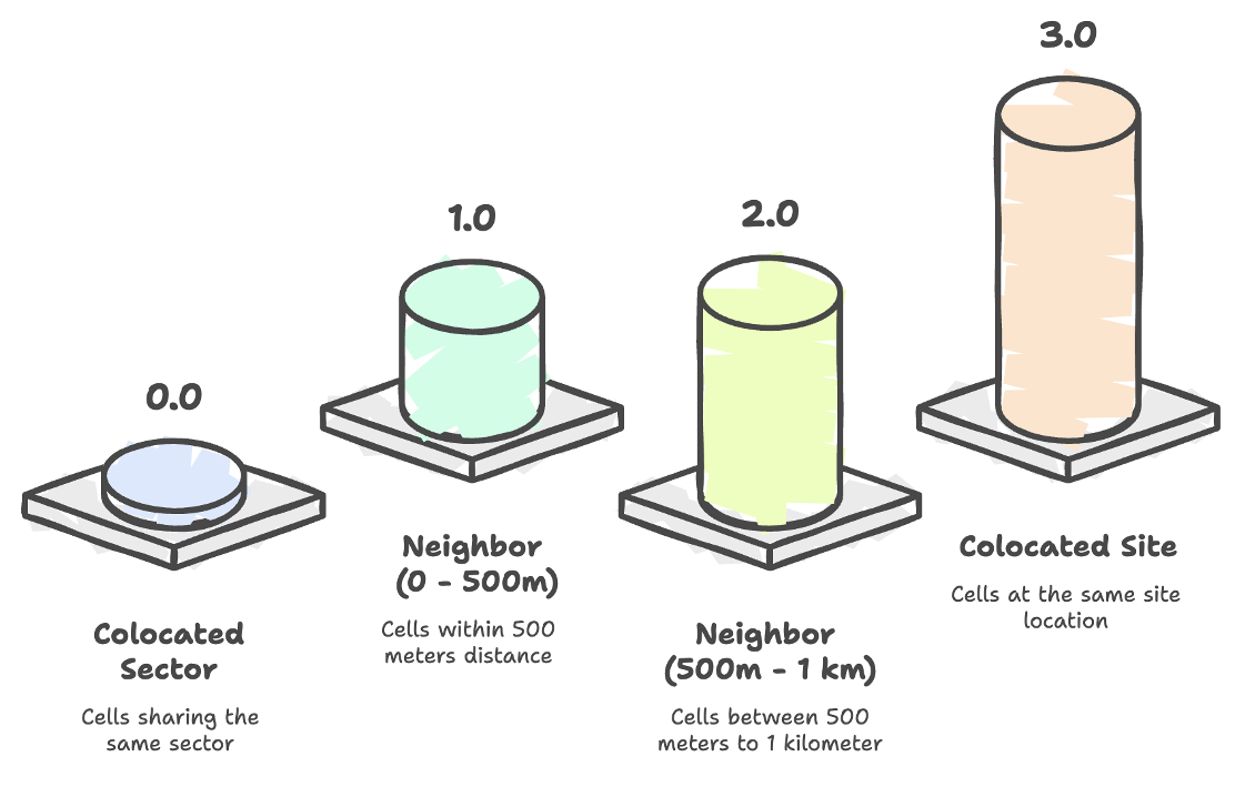
The Priority Model

I also wanted the result to be explainable. Instead of producing one opaque score per candidate, I classified the relationship and combined it with distance into four deterministic priority tiers:

Priority 0 — Collocated Sector Cell.
Priority 1 — Neighbor, 0 to 500 meters from the target.
Priority 2 — Neighbor, greater than 500 up to 1000 meters from the target.
Priority 3 — Collocated Site Cell.

An engineer looking at any row of output can trace exactly why it got the priority it did — which topology class it fell into, and which distance band, if it's a Neighbor. There's no hidden weighting to second-guess.

Priority model diagram: four tiers from Collocated Sector Cell (0) through Neighbor bands at 0–500m (1) and 500–1000m (2) up to Collocated Site Cell (3). — Every candidate that survives the direction check lands in exactly one of these four tiers — traceable back to topology and distance, not an opaque score.

def assign_priority(self, _df: pd.DataFrame):
    _df["Priority"] = _df["Destination Cell Type"].map(
        {"Colocated Sector Cell": 0, "Colocated Site Cell": 3}
    )

    conditions = [
        (_df["Destination Cell Type"] == "Neighbor")
        & (_df["Distance (m)"] >= 0)
        & (_df["Distance (m)"] <= 500),
        (_df["Destination Cell Type"] == "Neighbor")
        & (_df["Distance (m)"] > 500)
        & (_df["Distance (m)"] <= 1000),
    ]

    priority_values = [1, 2]

    _df["Priority"] = np.select(
        conditions,
        priority_values,
        default=_df["Priority"],
    )

    return _df

The actual priority-assignment step: Collocated Sector / Collocated Site cells get a fixed priority via a direct map, Neighbor cells get 1 or 2 depending on which distance band they fall into, applied over the whole candidate table at once with np.select rather than row by row.

Making It Operational

None of this was useful sitting in a notebook — it had to run as a daily pipeline that could refresh the neighbor database as the network changed. The flow is roughly: extract the current network configuration, compare it against the previous day's data, and only run the full candidate-generation and classification logic when something actually changed. Otherwise there's nothing new to compute.

When there are changes, it generates geographic candidates, classifies the relationships, eliminates candidates that fail the direction check, assigns priorities, and saves the output — which then gets backed up and handed off downstream.

I added a few safeguards once this moved from a one-off script to something that runs unattended every day: the previous output gets backed up before being overwritten, there's a post-check that flags it if records unexpectedly disappear between runs, errors get logged, failures trigger a notification, and where it applies the pipeline can fall back to the last good backup instead of shipping an empty or broken output.

Network configuration

Daily extraction

Change detection

Candidate generation

Direction validation

Topology / priority

Neighbor DB

Downstream consumption

Runs daily; the candidate-generation and classification steps only fire when the network configuration actually changed since the last run.

Checking It Visually

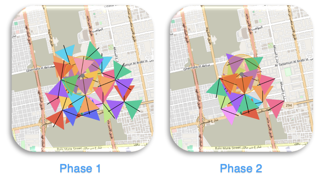
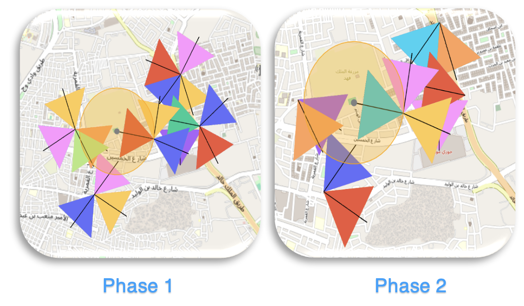
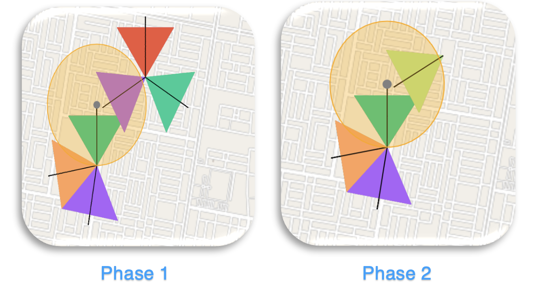
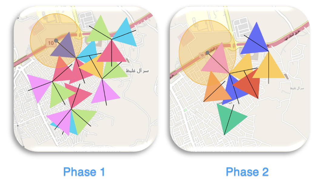
I didn't want to trust the geometry blindly, so I built a small visualization tool that renders the computed candidates and their classifications against real sector layouts. It draws each candidate's sector as a triangle at its actual bearing, along with the search radius around the target, so I could look at a case and immediately tell whether the direction-aware logic was doing something sensible.

I used it to compare, case by case, what the proximity-only candidate set looked like against what survived the direction-aware elimination. The four cases below are actual runs of that tool — each one already shows the before/after comparison for that case in a single frame.

Case 01 — Each case shows the proximity-only candidate set alongside what survived the direction-aware elimination, in the same frame.

Case 02 — Each case shows the proximity-only candidate set alongside what survived the direction-aware elimination, in the same frame.

Result

Candidate selection moved beyond distance-only logic — direction now has to agree with distance before a candidate qualifies.
Out-of-direction candidates get eliminated instead of silently sitting in the neighbor list.
Topology is explicit: collocated-sector, collocated-site, and neighbor are three different things, not one bucket.
Priorities are deterministic and explainable — four tiers, each traceable to topology and distance.
The output can be refreshed as the network configuration changes, instead of being a one-time computation.
The visualization tool gives an engineer a way to sanity-check the relationships instead of trusting the numbers blindly.

Downstream IT validation reported approximately 99% database accuracy.

Limitations & Trade-offs

The distance bands and the angular-alignment threshold are fixed, configurable parameters, not learned or adaptive values. That was a deliberate choice — I wanted the output to stay explainable, and a fixed rule you can point to beats a model whose reasoning you'd have to reverse-engineer.

That also means results are only as good as the underlying coordinate and antenna-azimuth data. If a site's azimuth is recorded wrong, the direction check will be wrong too, and no amount of geometry fixes that. The visualization tool is a verification aid, not a guarantee — whether it's wired into the live decisioning pipeline can vary by deployment stage.

Ask Me About

Why geographic proximity alone isn't enough for RAN neighbor relationships
Bearing vs. antenna azimuth — what the difference actually is and why both matter
How I compute angular alignment, and why I used a configurable threshold instead of a fixed one
The four-tier priority model, and how each tier maps back to topology and distance
How I used visual validation to sanity-check the geometry
Trade-offs of a fixed, rule-based model versus a learned or adaptive one